Renewable energy Hackathon

This was part of a hackathon hosted by the Imperial College Data Science Society (ICDSS).

Our code can be found on GitHub . The state of the repo at time of submission can be found in the releases. However, we were very tired/rushed from the Hackathon format so we have tried to clean up the repo, and have added a few more features since the hackathon.

Here I will run through our solution, and try and give a timeline for our progress throughout the 24 hours.

Our team consisted of:

The Problem

The energy supplied by renewables is sporadic, and has to be stored in batteries when the demand is low. It is then ready to sell to the customer when demand becomes high.

Now, the price of energy varies throughout the day, so the question is:

What strategy of charging/discharging will make the most profit over time?

Energy price

Initial data exploration showed that the price of energy was quite periodic/predictable throughout the day. This periodic nature is demonstrated in the figure below, where the price per day (for the entire 3 year dataset) is superposed onto the same axes. The large spikes in the afternoon are quite obvious in this figure, and could be something to exploit later in the project.

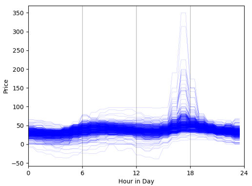
Superposed energy price per day in the entire dataset

Figure 1. Superposed energy price per day in the entire dataset. Spikes in the afternoon are interesting.

Our Solution

Our initial thought was some kind of structured charge/discharge cycle, i.e. pick points from Figure 1 and say every day we will charge/discharge here and hope that it follows the same pattern.

With such periodic data, this strategy would probably work, but it has some serious flaws and is not very flexible.

Since it was an AI hack, we turned our attention to machine learning (ML). This problem didn’t seem to fit into the classic ML problems of classification and regression that we have some basic knowledge of.

Although we are PhD students, we have no focus/link to ML, therefore we weren’t sure how to continue. We asked for a hint from the ICDSS, who suggested that reinforcement learning could be useful…

Reinforcement Learning

So what even is reinforcement learning?

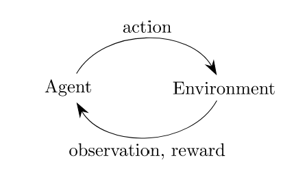
Using the “pole” example from OpenAI. We have an agent (the hand) who can take actions (left or right) in this environment (keeping a pole upright).

For each of these actions, we can reward the agent in the aim that they will learn a successful strategy. In this example, the reward will be the time that the pole is upright.

Pole environment

So to summarise we want to teach the agent how the maximise the reward.

Environment

In our case, we can adapt this example to our problem:

Agent

The agent is now our battery.

Actions

Buy (charging with some energy)
Hold (do nothing)
Sell (discharging some energy)

Reward

We now want to reward the agent for:

Selling when the price is high
Buying when the price is low

So achieve this we created a simple reward for each action that the agent took.

\[R = -\Delta E * (CP - EP),\]

where R is the reward, CP is the current price and EP is the expected price and \(\Delta E\) is the change in energy.

For example, if we are SELLING then we will be discharging, so \(\Delta E < 0\). If we sell when the price is higher than expected (\(CP - EP > 0\)) then we will have a positive reward (\(>0\)). If the price was lower than expected, then we would have a negative reward (\(<0\)), which is a punishment.

Expected Price

This simple reward function requires knowledge of the “expected price”. As we didn’t have much time, we have settled for a simple approach of taking the “median” average of the previous 24 hours. This does a good job of picking out the central part of the daily shape in Fig. 1. We originally used the “mean”, but this did a poor job when there was a spike in the energy price, as shown in Fig. 2. Ideally, we would have a much better estimate of “expected price”, using some kind of forecasting, which is discussed later.

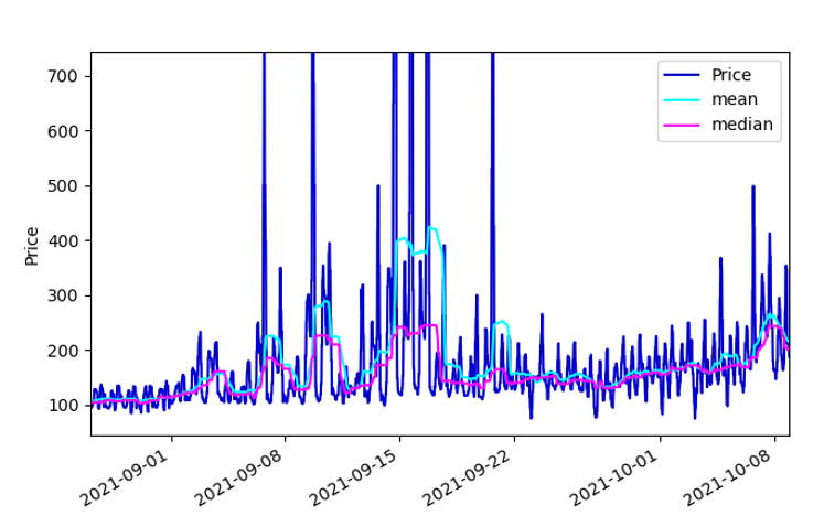
Comparison of mean and median average of the energy price

Fig. 2 Comparison of mean and median average of the energy price

Training the Model

Since we have systematically defined the reward, agent, actions, then we can use the base environment class from OpenAI’s Gym. This has the massive advantage of being compatible with OpenAI’s PPO algorithm through the Stable-baselines3 package. This was crucial as we could just write model.learn() and let the underlying Neural Network find a good strategy, which is not something we could have come up with in 24 hours!

Results

Before training

To demonstrate how well the training performs, we have shown the performance of an “un-trained” agent in Fig. 3. Here we can see that it just randomly takes actions, which results in a total reward centered around 0.

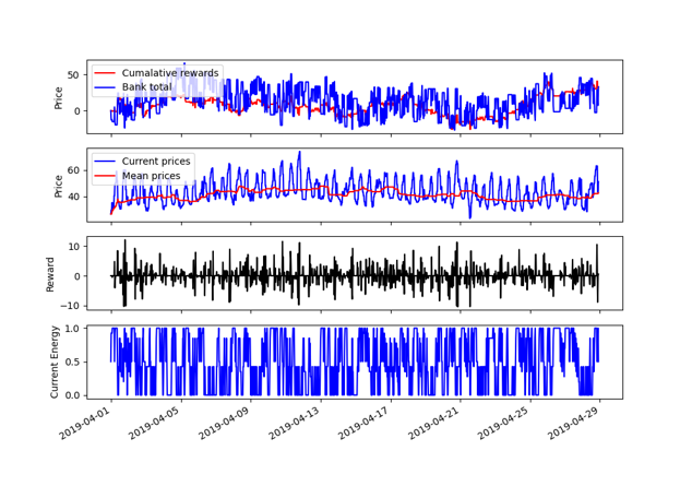
Agent performance before it is trained

Fig. 3: Agent choosing random actions before it is trained.

After training

After the training, we can see that it takes fewer buy or sell actions, and is making a steady profit. Over the entire 3 year period our model made £15,000 profit. We were really happy with this result, as it gave an increasing profit but with a solution that has lots of room for development.

Agent performance after training

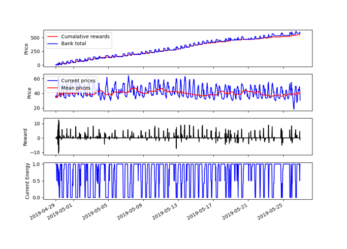
Fig. 4: Agent after training, where it takes a more succesfull strategy

Whole dataset

This is the final result on the whole dataset.

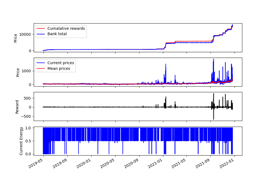
Fig. 5: Results over the whole dataset, with a profit of £15,000

Room for improvement

Selling too early

We noticed that our model would sell the instant that the “current price” went above the “expected price”. Although this does make a profit, it means that we run out of energy to sell before the maximum energy price of the peak.

We attempted to alter the reward by adding some kind of gradient of energy price, but could not get it to work in the time limit.

Just before submission we altered the discharging rate of the battery (by halving it). This allowed the model to make more sell actions before it ran out of charge. Such a simple change increased our profit by another £10,000 as seen below.

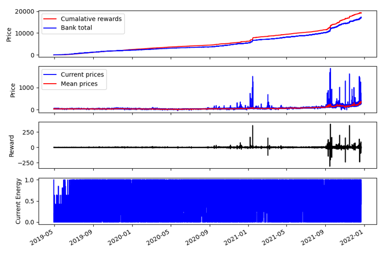
Effect of reducing the power output of the battery

Fig. 6: If we reduced the power output of the battery by half, we can greatly increase the profit over Fig. 5

This could be further improved by knowing a more accurate forecast of the energy price…

Expected Price

Ideally we would have a forecast of the energy price as our “expected price” instead of the median average. However, we did not have time to complete this as part of the Hackathon. We have since worked on a Bayesian forecasting technique, which looks promising.

Timeline

Before the Hackathon: We created a GitHub repo with a basic conda environment and pre-commits installed
11:30: Projects are announced. We chose the energy based project over the image based one. But we were unsure whether to focus on battery charging or forecasting the energy price.
12:00: Brainstormed potential solutions. For the battery aspect, we naively thought it could be solved through if/else statements.
12:30: Went to pick up freebies and pizza. Although, this took an hour to arrive!
14:00: Got the data loaded and parsed into pandas DataFrames.
17:00: Wasted a lot of time trying to sort out timezones (which we didn’t even use in the end). Also kept trying different solutions and researching forecasting models.
19:00: Got a bus from University back home, and used this as an opportunity to research Reinforcement learning.
21:00: Ate a curry and talked about the different Python packages we may need.
22:00: Installed PyTorch, Gym and stable-baselines3.
01:00: Created the Gym based environment for our agent to learn.
02:00: Started making the submission notebook.
02:20: Succesfully trained the model on a month of data.
03:00: Finished for the night with an ok model.
09:30: Changed mean to median which greatly improved the model.
10:00: Changed the way the model “saw” the data. This was a crucial structural change as we could give it a smaller array, which sped up learning.
11:00: Made final submission notebook
11:30: Tried to make a video presentation, but ran out of time. Just rick rolled the judges instead…
13:30: The plan said winners would give a presentation now. But the schedule was changed.
13:40: Told we would be giving a presentation at 14:30
14:30: Quickly made a presentation.
15:00: Phil gave an incredible presentation that receieved very positive feeback.
16:00: Winners announced! (🎉)